The history of quantitative analysis goes back far before computers, and this work leads directly into how the field progresses once computers can be applied. In this first post we explore the history and development of quantitative analysis as it applied to finance in the pre-computer world of the early through mid 20th century.
Actively managed ETFs are dominating new launches. However, the vast preponderance of assets remain in ETFs managed through quantitative investment modeling and dominated by index funds in particular. What many people don’t know is that the roots of such investing approaches came many years before the 1940 Investment Act governing mutual funds and well before the dawn of computers.
All 5,000 stocks, 16 sector groups, 140 industries, and 500 ETFs have been updated: Two-week free trial: www.ValuEngine.com
Let’s start with a couple of working definitions:
Quantitative investment models offer a systematic and data-driven approach to investment strategies in financial markets. Quantitative investment management may loosely be described as the application of rigorous mathematical models and statistical principles, informed by economic theory, to the study of financial markets with the primary goal of selecting stocks and constructing investment portfolios.
This diagram depicts an overview of components common to most quantitative investment models:
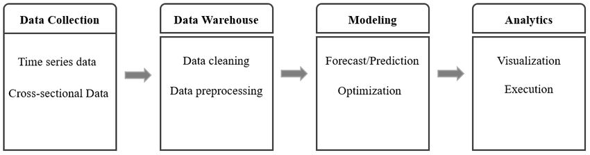
- The data series used in modeling must generally have two dimensions: a) They must be values recorded at regular intervals across time, referred to as time series and b) they must constitute a typical or representative sample of a larger group referred to as a cross-sectional sample.
- Whether this data is being collected from historical records, culled from surveys, scraped from the web or some other alternative source, they must be cleaned and processed before modeling.
- The modeling itself requires a methodology. The modeling technique used should be carefully selected to be appropriate for its purpose.
- Along with the model’s results, it is important to provide analytics that explain what the results mean and the size of potential estimation errors.
Current ValuEngine reports on all covered stocks and ETFS can be viewed HERE
With the basic construct of quantitative investment modeling now broadly defined, the beginning of most models used in the 20th Century and beyond started with a master’s thesis by Louis Bachelier in 1900. The original title in French was “Théorie de la Spéculation” (Theory of Speculation) 1900.
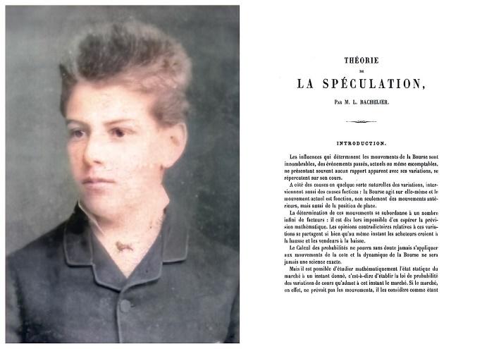
In mathematical terms, Bachelier’s achievement was to introduce the physics concept of Brownian motion, small random fluctuations, to stock price movements. His immediate purpose was to give a theory for the valuation of financial options. This was more than 70 years ahead of the Black-Scholes model for options valuation. Nevertheless, this landmark thesis was resurrected by Harry Markowitz in 1953 and William Sharpe in 1964 to provide the underpinnings of Modern Portfolio Theory.
The major achievement in the annals of the progress of quantitative investment research was also born in a master’s thesis. Somewhat paradoxically, this came during The Great Depression and the global build-up to World War II. Even though the US stayed clear of the war for three more years, almost everyone in the country was talking about it.
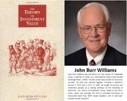
The research in question was John Burr Williams and the year was 1938. Dr. Williams was a security analyst who sought a better understanding of what caused the stock market crash of 1929 and the subsequent Great Depression. He enrolled as a PhD student at Harvard and his thesis, which was to explore the intrinsic value of common stock, was published as The Theory of Investment Value. Williams proposed that the value of an asset should be calculated using “evaluation by the rule of present worth”. Thus, for a common stock, the intrinsic, long-term worth is the present value of its future net cash flows—in the form of dividend distributions and selling price. Eventually, The Theory of Investment Value was published as a book and is still being sold today.
1938 also saw the beginnings of an economic research study that would later become one of the most important linchpins of quantitative investing today. Alfred Cowles established the Cowles Commission for Research in Economics six years earlier. The Commission’s motto “Science is Measurement” turned out to be quite prophetic indeed. In need of a measurement stick, Cowles created a market index. For the index, he aggregated the sum of the products of the closing price times the shares outstanding of every stock traded on the New York Stock Exchange. This was very laborious manual work done with only the aid of an adding machine. The idea was to capture the daily fund flows in the US Stock Market for econometric purposes. He considered this to be more representative of the average investors’ experience than any of the Dow Jones Averages. The comparison proved apt because it was the continuing Cowles Commission research and index, sold to Standard & Poor’s in 1957, that later grew to be the S&P 500 Index.
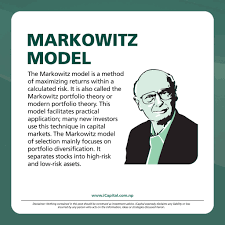
Let’s skip another 14 years from 1938 to a PhD dissertation by Harry Markowitz. It was named simply – “Portfolio Selection” (1952). 12 years later, no less an authority than William Sharpe, Ph.D. would characterize it as the seminal document laying out the underpinnings of Modern Portfolio Theory. The paper introduced the concept of optimizing portfolio diversification in an effort to lower portfolio risk (variance) without sacrificing return.
Current ValuEngine reports on these stocks or ETFS can be viewed HERE
The Markowitz model of portfolio suggests that the risks can be minimized through diversification. Simultaneously, the model assures maximization of overall portfolio returns. Investors are presented with two types of stocks—low-risk, low-return, and high-risk, high-return stocks. It introduced the concept of paired covariances rather than correlation coefficients for each pair of stocks in the portfolio.
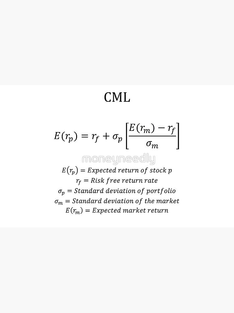
The Markowitz formula is as follows:
RP = IRF + (RM – IRF) * σP/σM
Here, RP = Expected Portfolio Return; RM = Market Portfolio Return;
IRF = Risk-free Rate of Interest; σM = Market’s Standard Deviation;
σP = Standard Deviation of Portfolio
Many people consider the recently deceased Dr. Markowitz as the father of modern quantitative investing. Again, this concept was more theoretical than anything that was implementable by practitioners. The computing ability that was available in the 1950’s simply could not handle all the required calculations for a portfolio of 30 stocks or more.
In the early 1960’s, a number of interesting papers were written by soon-to-be very important people in quant finance including work on the Efficient Market Hypothesis and theories that stock prices move in a random walk, building on Bachelier’s application of Brownian motion to stock prices. Dr. Jack Treynor and Dr. Paul Samuelson are just two of the authors writing during this period.
That said, I consider William Sharpe’s “Portfolio Selection” in 1964 to be the next major event in the advancement of quantitative investing. It was his exposition of the underpinnings of Modern Portfolio Theory that really put the concept on the map. The article forever changed the curricula for students in finance throughout academia, starting with the University of Chicago and soon including Harvard, Yale, Cal-Berkeley and Stanford. After that it was mainstream teaching in almost all business schools in the United States.
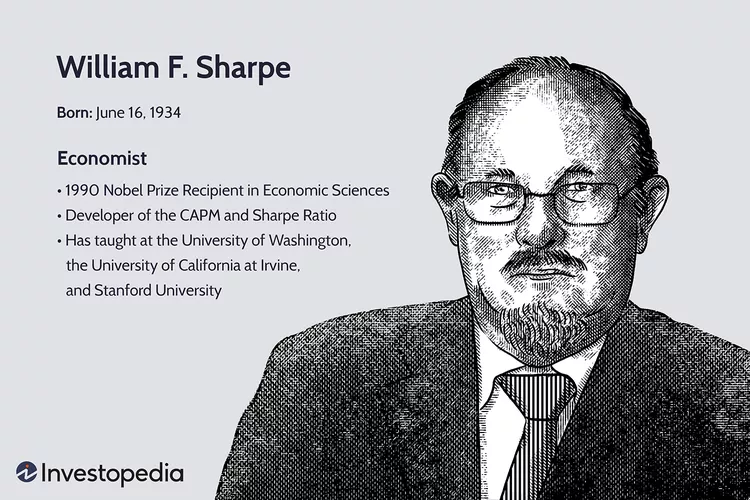
“Portfolio Selection” introduces the Capital Asset Pricing Model. The CAPM is a cornerstone in portfolio management and seeks to find the expected return by looking at the risk-free rate, beta, and market risk premium.
CAPM Formula
Calculate the expected return of an asset, given its risk, is:
𝐸𝑅𝑖=𝑅𝑓+𝛽𝑖 * (𝐸𝑅𝑚−𝑅𝑓) where:
𝐸𝑅𝑖=expected return of investment; 𝐸𝑅𝑖=expected return of market;
𝑅𝑓=risk-free rate; 𝛽𝑖=beta of the investment; (𝐸𝑅𝑚−𝑅𝑓) = market risk premium
From this formula the formula for the Capital Market Line (CML) is derived.
Dr. Sharpe’s next major contribution, still used today, was the creation of the Sharpe Ratio. The Sharpe ratio helps investors evaluate which investments provide better returns per risk level.
Sharpe Ratio= (Rp−Rf) / σp
where:
Rp = return of portfolio Rf=risk-free rate
σp = standard deviation of the portfolio’s excess return
Many of Sharpe’s new constructs became the new focus of academia. This includes two 1965 efforts to advance the Efficient Market Hypothesis.
In 1965, Paul Samuelson, PhD (1965) (right pic) expanded on Bachelier’s earlier work. He published a proof showing that if the market is efficient, prices will exhibit random-walk behavior…However, from a practical application perspective, “a nonempirical base of axioms does not yield empirical results.”
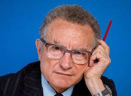

Samuelson Fama
Eugene Fama’s dissertation (1965): An ‘efficient’ market is defined as a market where there are large numbers of rational profit-maximizers actively competing, with each trying to predict future market values of individual securities, and where important current information is almost freely available to all participants.”
Financial Advisory Services based on ValuEngine research available: www.ValuEngineCapital.com
Random Walk Asset Pricing Defined
Mu is a drift constant; Sigma is the standard deviation of the returns;
Delta{t} is the change in time; Y-sub-I is an independent and identically distributed random variable between 0 and 1.
All of these were theoretical contributions to the underpinnings of quantitative investment research. By the mid-1960’s, it was being taught in academia but not implemented as of yet for a variety of reasons including, but not limited to, lack of sufficient computing power. All that would change soon.
This journey through the past to the present will continue in next week’s blog chapter with the progression of quantitative analysis through the computer age.
_______________________________________________________________
By Herbert Blank
Senior Quantitative Analyst, ValuEngine Inc
www.ValuEngine.com
support@ValuEngine.com
All of the over 5,000 stocks, 16 sector groups, over 250 industries, and 600 ETFs have been updated on www.ValuEngine.com
Financial Advisory Services based on ValuEngine research available through ValuEngine Capital Management, LLC
Free Two-Week Trial to all 5,000 plus equities covered by ValuEngine HERE
Subscribers log in HERE