Part I of this article (posted on Blog.ValuEngine.com on May 22, click HERE) started with Louis Bachelier’s work from 1900 and covered all the theoretical work done up to and including William Sharpe, Ph.D.’s seminal work in 1964. However, none of that early research had yet been applied successfully to actual investments in any meaningful way. The next 60 years reflect the application of these historical and new quantitative processes with the use of computers. The field moves forward even more quickly once computing power is applied.
Empirical Research and Implementation:
Much changed in 1965. Sam Eisenstadt (1965), Director of Research for a well-known encyclopedic subscription publication called Value Line, created what became known as the Timeliness Ranking System. It was the culmination of five painstaking years of research.
All 5,000 stocks, 16 sector groups, 140 industries, and 500 ETFs have been updated:
Two-week free trial: www.ValuEngine.com
The Value Line Timeliness rank measures probable relative price performance of the approximately 1,700 stocks during the next six months on an easy-to-understand scale from 1 (Highest) to 5 (Lowest). The components of the Timeliness Ranking System are the 10-year relative ranking of earnings and prices, recent earnings and price changes, and earnings surprises. All data are actual and known. Regression equations refit the coefficients of each of the 5 variables quarterly.
Ranks based on relative scores imitating standard bell curve.
Top 100 = Group 1; Next 300 = Group 2; Next 900 = Group 3;
Next 300 = Group 4; Bottom 100 = Group 5.
Unlike its theoretical predecessors, these ranks were used immediately by some asset managers and private investors as part of their input processes. Mr. Eisenstadt said, “Empirically, future stock prices are not determined by Beta but by dynamic combinations of earnings- and price-related values.” This was disputed by noted economist and University of Chicago Business School Professor Fischer Black. He asked for all of the system’s historical raw data and wanted to see if he could duplicate the results for himself. He did and wrote an academic paper in 1973 verifying that the Timeliness Ranking System was an “anomaly”, a rare exception to the Efficient Market Theory. This concept of an accepted anomaly by academia paved the way for empirical anomalies discovered in the future to be used in asset management processes.

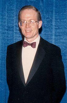
Sam Eisenstadt Fischer Black
Taking Index Investing from Theory to Reality:
Meanwhile, efforts to apply Modern Portfolio Theory to managing portfolios persisted at Wells Fargo Asset Management under the aegis of John McQuown, an MPT advocate. He was charged with exhaustive research to create an asset management strategy that would outperform random portfolios. He empirically concluded after testing all data he accumulated for three years and backtested over 10 years before that – all using punch card data entry – that it was impossible to systematically succeed. He concluded that the random walk theory was the best one for the project to use. He wanted to create and manage the world’s first index fund and hired another MPT advocate, William Fouse, to help him. The project took on life when real money was proffered from a pension fund investor.
Current ValuEngine reports on all covered stocks and ETFS can be viewed HERE
University of Chicago Professor Keith Shwayder, a scion of the family that owned Samsonite and a big believer in Modern Portfolio Theory, was intrigued enough by the idea that he committed six million dollars from the firm’s pension fund to invest in the entire market. The question was how to implement it. Helped by William Fouse and James Vertin, they started by believing that to index the entire market the best solution was to buy an equal amount in every stock traded on the New York Stock Exchange and rebalance to equal every day using the computer. This was a disaster. It was 1971 and transaction costs were much higher than they are today and they lost 15% of the value of the fund in the first week on frictional costs alone. It was then that McQuown and Fouse discovered the S&P 400 (now 500) Index and were invited to index that. Success – portfolio needed little rebalancing since weightings moved with index weightings. Transaction costs minimized. Many institutional money managers and pension funds quickly followed suit.

John McQuown William Fouse
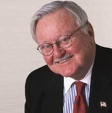
Perhaps an even greater factor in the success of index funds was John (“Jack”) Bogle, Founder of Vanguard Funds. In fact, many people are under the impression that he created the first Index Fund. This is an oft-repeated yet erroneous assertion. He was neither an academic nor a mathematician. In the mid-1970s, as he started Vanguard, he was analyzing mutual fund performance, and he came to the realization that “active funds underperformed the S&P 500 index on an average pre-tax margin by 1.5 percent”. He also found that this shortfall was virtually identical to the costs incurred by fund investors during that period.
This was Bogle’s a-ha moment. He started the first index mutual fund based upon the S&P 500 and licensed the index from S&P, starting a new business model for the latter. “Bogle’s Folly”, as it was called by disdainful competitors, stood alone in offering low-cost unmanaged equity exposure to fund shareholders for the next 20+ years. So, while Jack didn’t invent index fund investing, he certainly democratized it and popularized it.

Jack Bogle
Options Theory Research – a Foundation for Subsequent Fixed Income and Equity Studies:
The next major quantitative breakthrough from my perspective came from expanding Bachelier’s contribution to options theory. The Black-Scholes call option formula is calculated by multiplying the stock price by the cumulative standard normal probability distribution function. Thereafter, the net present value (NPV) of the strike price multiplied by the cumulative standard normal distribution is subtracted from the resulting value of the previous calculation. Economist Robert Merton coined the term the “Black-Scholes” model and authored the published paper that gained it fame in The Journal of Financial Economics in 1975.
In mathematical notation, the formula is:
Because this model has several restrictive and non-real-world assumptions attached to it, some subsequent options pricing models have been proposed and used, most notably Cox-Ross-Rubenstein in 1979. The beauty of the generalized Black-Scholes equation on which the formula is based is that it can be applied to any asset.

Myron Scholes Fischer Black Robert Merton
Decomposing Beta into the market factor plus other systematic factors contributing to equity risk:
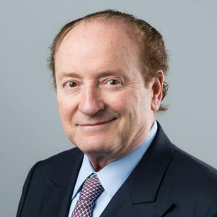
The next major mathematical contribution to asset management came from Dr. Stephen Ross of Yale University in 1976. He proposed the Arbitrage Pricing Theory (1975) showing that Beta was an oversimplification. He demonstrated that risk was decomposed to economic factors such as GDP, term structure of interest rates, inflation, etc. The formula was expressed:
E(R)i=E(R)z+(E(I)−E(R)z)×βn
where: E(R)i=Expected return on the asset;
Rz=Risk-free rate of return;
βn=Sensitivity of the asset price to macroeconomic factor
nEi=Risk premium associated with factor i
A major contribution from the decomposition of market risk into component factors was the ability to better optimize portfolios. This was taken further by Barr Rosenberg (1976), the founder of BARRA. In lieu of economic factors, Rosenberg substituted fundamental factors. Many industry professionals found these risk explanations for stocks to be much more consistent with their expectations of how the market works. Beyond this, as better computer power became available, Rosenberg directed the construction of optimizers that would take multiple security factor exposure of hundreds of stocks at a time to create portfolios designed to maximize the expected-return-to-unit-of-risk ratios.
Stephen Ross
Exploiting anomalies – the foundations of active quantitative investment management:
From these breakthroughs, the dawn of the active quantitative investment management era emerged in the late 1970’s. In the 1980’s, it became more than academic as institutionally oriented quantitative investment management first began to proliferate. This phenomenon coincided with the publication of academic research studies based upon empirical anomalies to the Efficient Market Theory. Explanations for these anomalies have been debated in academic literature but common themes are: mispricing; unmeasured risk; selection bias; imperfect information discovery; frictional costs; and limits to arbitrage.
Anomaly studies include but are not limited to works such as:
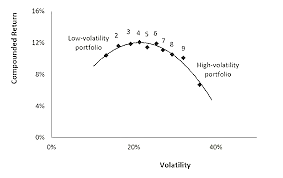
Haugen, Robert A., and A. James Heins (1975), “Risk and the Rate of Return on Financial Assets: Some Old Wine in New Bottles.” Journal of Financial and Quantitative Analysis; often called the low-volatility anomaly, this article demonstrated that the relationship between Beta and future price does not hold for the higher side of the spectrum. That is, stocks with Betas of 1.5 do not systematically return 50% more than stocks with Betas of 1.00 demonstrating that investors are not adequately compensated for assuming added volatility risk.

Robert Haugen
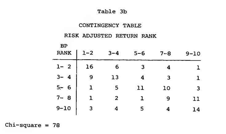
“Book Values and Stock Returns” by Dennis Stattman in The Chicago MBA: A Journal of Selected Papers (1980). I could not find a picture of Stattman but found this table illustrating the anomaly in his seminal work. This documented the fact that during the time period measured, stocks with low book-to-price ratios (e.g, high price/book) underperformed stocks with high book-to-price ratios.
“The Relationship Between a Stock’s Total Market Value and Its Return” by Rolf Banz in the Journal of Financial Economics (1981); this was the first documented article on the small-cap stock anomaly.

Rolf Banz
The next group of “anomalies” is included to better understand the evolution of quantitative asset management but they were used more sporadically if at all when compared with the above anomalies.
“Earnings Releases, Anomalies, and the Behavior of Security Returns” by George Foster, Chris Olsen and Terry Shevlin in The Accounting Review – Journal of the American Accounting Association (1984). For many years, this was called the earnings surprise anomaly. The remainder of the 1980s saw a plethora of research papers documenting empirical anomalies with “factors” such as “Momentum Reversal”, “January Effect”, “Dogs of the Dow”, “Bid-Ask Spread”, “Weekend Effect”, “Market Leverage” and “Short Term Reversal.” These “factors” are still used by individual investors and smaller portfolio managers but are not recognized as factors today by the institutional investment communities.
Current ValuEngine reports on all covered stocks and ETFS can be viewed HERE
Many active quantitative asset managers used some combination of the above anomalies on either a strategic or tactical basis. In conjunction with various ranking systems by research departments and optimizers, the results were highly diversified portfolios for pension funds and other institutions. However, in most cases the promise of outperformance by the anomaly “factors” did not translate into outperforming portfolios with respect to their institutional benchmarks. A common lamentation was that the process including frictional costs from turnover optimized the alpha away.
However, while not outperforming the benchmark indexes as a group, the results for quantitative active management firms in the aggregate were superior enough to traditional active managers that they became a staple for the recommendations of pension fund industry consultants. This led to the question of what active management and manager skill, if anything, could active managers, both quantitative and traditional, add to investment returns.
The fundamental law of active management:
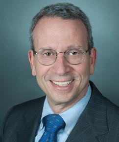
What could active managers add to investment returns? This basic question was addressed in the seminal article, “Fundamental Law of Active Management” published in the Journal of Portfolio Management (Spring, 1989) by Richard Grinold. The article focuses on an Information Ratio by modifying the Sharpe Ratio formula by substituting the active portfolio’s benchmark index returns for the risk-free rate of returns. The “law” asserts that the maximum attainable Information Ratio (IR) is the product of the Information Coefficient (IC) times the square root of the breadth (BR) of the strategy. Subsequent iterations led to articles and books published jointly by Grinold and another professor, Ron Kahn.


Richard Grinold Ron Kahn
Five common systematic risk factors determining stock and bond returns:
The next seminal article on systematic factors that active managers could potentially use to improve quantitative performance came from noted quantitative giants’ Eugene Fama and Kenneth French. Both were early proponents of the Strong Form of Efficient Market Hypothesis and Modern Portfolio Theory espousing that it was impossible for active managers to systematically beat the market because stock prices change in a manner approximating a random walk distribution. Bolstered by meticulous empirical studies, they published a study that has since become a major backbone of most quantitative investing practices. The study was called “Common risk factors in the returns on stocks and bonds” and published in the Journal of Financial Economics (1993). The study includes citations from nearly all the authors listed in this paper and from a practical applications perspective laid the groundwork for all to follow in this third phase of the quantitative investment management evolution.
In short, This paper identifies five common risk factors in the returns on stocks and bonds. There are three stock-market and overall market factors related to firm size and book-to-market equity. There are two bond-market factors. shared variation due to the stock-market in the bond-market related to maturity and default risks. Stock returns have factors, and they are linked to bond returns through corporate bonds, principally with high-yield bonds. The five factors seem to explain average returns on stocks and bonds:
The stock market factors include:
- Market Factor – the residual Arbitrage Pricing Theory Beta after accounting for other verified factors;
- Size Factor as measured by market capitalization;
- Value Factor as defined by the ratio of book value to market capitalization.
The bond factors include:
- Term structure risk; and
- Default risk.
I include an explanation of the entire model because price movements and risk exposure of equities and bonds are intertwined in the capital markets although the nature of that relationship changes with time. A more direct relationship was observed in this paper with high-yield (or low quality) bonds. This later led to research that a quality risk factor, generally defined as a combination of financial strength and earnings consistency, also exists and further increases multi-factor explanatory power. The firm they helped found, Dimensional Fund Advisors, uses all of these factors in its quantitative active management processes.

Image of Eugene Fama with Kenneth French from Dimensional Fund Advisors’ Website
Three-factor quantitative modeling requiring stochastic techniques:
Most of the above research was referenced either explicitly or implicitly in the research paper, “Stock Valuation in Dynamic Economies” by Gurdip Bakshi and Zhiwu Chen from the Yale International Center for Finance (2001). The two professors had previously been best known for an options-pricing article published in the Journal of Finance in 1997 entitled “Empirical Performance of Alternative Option Pricing Models.”
The Yale article develops and empirically implements a stock valuation model. The model proposes a
stock valuation formula that has three variables as input:
- net earnings-per-share;
- expected earnings growth, and;
- forecasted interest rate.
Using a sample of individual stocks, the study demonstrates the following results:
- Modeling expected earnings growth correctly requires stochastic and non-linear processes with differing weighting schemes that depend upon each stock’s related industry sector;
- The derived valuation produces significantly lower pricing errors than existing models;
- A review of the information coefficients led to the conclusion that successful modeling of earnings growth dynamics is the key factor in achieving positive information ratios.


Gurdip Bakshi Zhiwu Chen
This article is my personal favorite. Among other reasons, that is because Professors Bakshi and Chen created the ValuEngine models and originally founded the firm to create independent stock ratings based upon them. ValuEngine therefore represents the practical application of a hundred years of advancements in quantitative financial research, applied on a daily basis and made available to individual investors and professionals.
ETFs raise the opportunities and importance of quantitative investment management techniques:
The twenty plus years since this article by Bakshi and Chen has seen both indexing and active quantitative investment management increase exponentially in importance to US investors. One key factor in the quantum leap in popularity has been the creation of exchange-traded funds or ETFs. Anyone who knows me knows this is another subject near and dear to my heart since I was the first US portfolio manager of ETFs with Deutsche Bank in 1996. Beyond that, I spent the next dozen years helping to popularize the efficiencies, utilities and versatility of the structural advantages in ETFs ever since that ETF family was launched. There is an article on the ValuEngine website that I authored explaining the structural advantages and their importance. That article was a 20-years-later follow-up to an article I had published in the Journal of Indexing in 2001 called “How ETFs Can Benefit Active Managers.” Changing the status quo is a tremendous challenge, but the ETF structure is so superior for so many in investing that 23 years later I defy anyone to say we didn’t pull it off.
“Smart Beta”
Meanwhile, quantitative asset management funds and ETFs have had their successes and failures. Rob Arnott founded the firm Research Affiliates and created the term “Smart Beta” to refer to schemes weighted by fundamental factors such as the ones documented by Fama and French. He teamed with a niche ETF provider to create RAFI (Research Affiliates Fundamental Indexes) ETFs in 2006. The funds outperformed their cap-weighted rivals in 2006 and 2007, leading to more industry attention and followers of the new paradigm. Then the financial crisis and the subsequent huge recovery happened. For many reasons, the result was that RAFI Indexes performed miserably compared to the S&P 500 in the next several years and the ETFs eventually were closed. As with many such concepts, fundamental indexing in various forms, including individual and combined “Smart Beta” factor investing has not died, it has simply been repackaged and is still used for many ETFs and other investment products in use today.

Rob Arnott
The fault lies both in the stars AND ourselves:
The underperformance of the original RAFI ETFs is not unique. Many active and passive quantitative investment products have underperformed prior data studies and simulations after being launched; most after enjoying initial success. Although backtests are met with sometimes-deserved skepticism, most of the people of the caliber included in this blog article painstakingly try to avoid selection and look-ahead biases among other common pitfalls. My 40+ years of experience in quantitative investment management lead me to the conclusion that all results in quantitative economic and financial studies are time period dependent. Markets are cyclical. There are many statistical methods for removing seasonality and cyclical dependency from quantitative testing. None of them are foolproof to put them mildly. Intrinsic cyclicality, almost by definition, means that some technique that produced extraordinarily good results during some randomly selected ten, twenty or even 100-year period will produce extraordinarily bad results in some other period of equivalent length. Even including the entire gamut of security returns from the history of investing would not solve this problem because if a method works overall but doesn’t work in nearly half the ten-year cycles, it is not helpful to most investors. Very few of us have 200-year investment horizons.
That fact conceded, all of the research above is very valuable in capital markets investing. One statistic that is abundantly clear as measured over time by nearly all researchers is that disciplined investment management methods such as active quantitative and indexing will minimize underperformance compared to traditional active techniques over time. The entire emphasis of all the research above is on identifying risk exposures. Trying to then apply those findings to asset management in predicting what will happen in the future is much less scientific as there are far more unknown variables and developing dynamics. Using quantitative methods is also a key to understanding what went right and wrong and whether adjustments need to be made.
Financial Advisory Services based on ValuEngine research available: www.ValuEngineCapital.com
I have a few more caveats. There are many other significant quantitative researchers and papers I did not touch upon here. If I attempted to list them, I’d more than double the size of this exercise. Also, in terms of the quantitative investing evolution, I’ve only barely touched on a couple of fixed income and options models and haven’t covered futures, structured products, cryptocurrencies and of the many other types of capital markets instruments at all. All of these arguably are even more mathematical and require more sophisticated modeling than the equity markets. Also, almost everything I’ve written in this series after covering Bachelier has been US-market-centric. Many important quantitative investment research efforts began and evolved in other countries.
Hopefully, many of you have found this two-part article to be helpful. All observations and comments I receive will be answered and may be used as the basis of a follow-up. Thank you for taking the time to read all of this.
_______________________________________________________________
By Herbert Blank
Senior Quantitative Analyst, ValuEngine Inc
www.ValuEngine.com
support@ValuEngine.com
All of the over 5,000 stocks, 16 sector groups, over 250 industries, and 600 ETFs have been updated on www.ValuEngine.com
Financial Advisory Services based on ValuEngine research available through ValuEngine Capital Management, LLC
Free Two-Week Trial to all 5,000 plus equities covered by ValuEngine HERE
Subscribers log in HERE